Visual Odmetry from scratch - A tutorial for beginners

I made a post regarding Visual Odometry several months ago, but never followed it up with a post on the actual work that I did. I am hoping that this blog post will serve as a starting point for beginners looking to implement a Visual Odometry system for their robots. I will basically present the algorithm described in the paper Real-Time Stereo Visual Odometry for Autonomous Ground Vehicles(Howard2008), with some of my own changes. It’s a somewhat old paper, but very easy to understand, which is why I used it for my very first implementation. The MATLAB source code for the same is available on github.

What is odometry?

Have you seen that little gadget on a car’s dashboard that tells you how much distance the car has travelled? It’s called an odometer. It (probably) measures the number of rotations that the wheel is undergoing, and multiplies that by the circumference to get an estimate of the distance travlled by the car. Odometry in Robotics is a more general term, and often refers to estimating not only the distance traveled, but the entire trajectory of a moving robot. So for every time instance \(t\), there is a vector \([ x^{t} y^{t} z^{t} \alpha^{t} \beta^{t} \gamma^{t}]\) which describes the complete pose of the robot at that instance. Note that \(\alpha^{t}, \beta^{t}, \gamma^{t}\) here are the euler angles, while \(x^{t}, y^{t} ,z^{t}\) are caetesian coordinates of the robot.

What’s visual odometry?

There are more than one ways to determine the trajectory of a moving robot, but the one that we will focus on in this blog post is called Visual Odometry. In this approach we have a camera (or an array of cameras) rigidly attached to a moving object (such as a car or a robot), and our job is to construct a 6-DOF trajectory using the video stream coming from this camera(s). When we are using just one camera, it’s called Monocular Visual Odometry. When we’re using two (or more) cameras, it’s refered to as Stereo Visual Odometry.

Why stereo, or why monocular?

There are certain advantages and disadvantages associated with both the stereo and the monocular scheme of things, and I’ll briefly describe some of the main ones here. (Note that this blog post will only concentrate on stereo as of now, but I might document and post my monocular implementation also). The advantage of stereo is that you can estimate the exact trajectory, while in monocular you can only estimate the trajectory, unique only up to a scale factor. So, in monocular VO, you can only say that you moved one unit in x, two units in y, and so on, while in stereo, you can say that you moved one meter in x, two meters in y, and so on. Also, stereo VO is usually much more robust (due to more data being available). But, in cases where the distance of the objects from the camera are too high ( as compared to the distance between to the two cameras of the stereo system), the stereo case degenerates to the monocular case. So, let’s say you have a very small robot (like the robobees), then it’s useless to have a stereo system, and you would be much better off with a monocular VO algorithm like SVO. Alos, there’s a general trend of drones becoming smaller and smaller, so groups like those of Davide Scaramuzza are now focusing more on monocular VO approaches (or so he said in a talk that I happened to attend).

Enough english, let’s talk math now

Formulation of the problem

Input

We have a stream of (grayscale/color) images coming from a pair of cameras. Let the left and right frames, captured at time t and t+1 be referred to as \(\mathit{I}_l^t\), \(\mathit{I}_r^t\), \(\mathit{I}_l^{t+1}\), \(\mathit{I}_r^{t+1}\). We have prior knowledge of all the intrinsic as well as extrinsic calibration parameters of the stereo rig, obtained via any one of the numerous stereo calibration algorithms available.

Output

For every pair of stereo images, we need to find the rotation matrix \(R\) and the translation vector \(t\), which describes the motion of the vehicle between the two frames.

The algorithm

An outline:

1. Capture images: \(\mathit{I}_l^t\), \(\mathit{I}_r^t\), \(\mathit{I}_l^{t+1}\), \(\mathit{I}_r^{t+1}\)

2. Undistort, Rectify the above images.

3. Compute the disparity map \(\mathit{D}^t\) from \(\mathit{I}_l^t\), \(\mathit{I}_r^t\) and the map \(\mathit{D}^{t+1}\) from \(\mathit{I}_l^{t+1}\), \(\mathit{I}_r^{t+1}\).

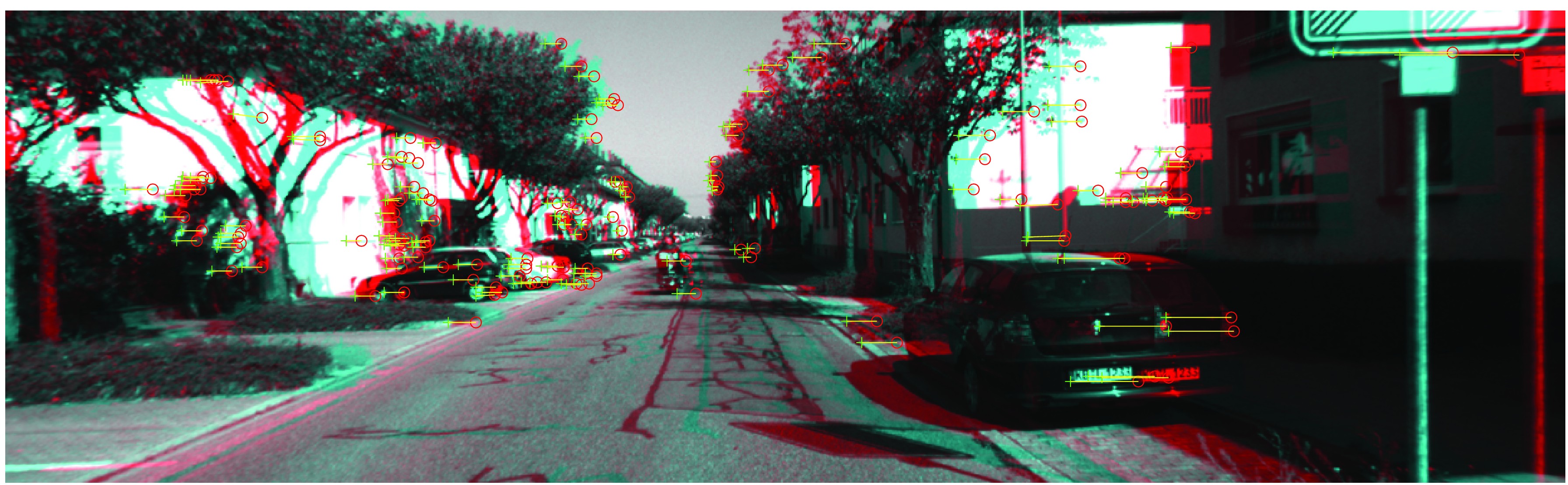
4. Use FAST algorithm to detect features in \(\mathit{I}_l^t\), \(\mathit{I}_l^{t+1}\) and match them.

5. Use the disparity maps \(\mathit{D}^t\), \(\mathit{D}^{t+1}\) to calculate the 3D posistions of the features detected in the previous steps. Two point Clouds \(\mathcal{W}^{t}\), \(\mathcal{W}^{t+1}\) will be obtained

6. Select a subset of points from the above point cloud such that all the matches are mutually compatible.

7. Estimate \(R, t\) from the inliers that were detected in the previous step.

Do not worry if you do not understand some of the terminologies like disparity maps or FAST features that you see above. Most of them will be explained in greater detail in the text to follow, along with the code to use them in MATLAB.

Undistortion, Rectification

Before computing the disparity maps, we must perform a number of preprocessing steps.

Undistrortion: This step compensates for lens distortion. It is performed with the help of the distortion parameters that were obtained during calibration.

Rectification: This step is performed so as to ease up the problem of disparity map computation. After this step, all the epipolar lines become parallel to the horizontal, and the disparity computation step needs to perform its search for matching blocks only in one direction.

Both of these operations are implemented in MATLAB, and since the KITTI Visual Odometry dataset that I used in my implmentation already has these operations implemented, you won’t find the code for them in my implmenation. You can see how to use these functions here and here. Note that you need the Computer Vision Toolbox, and MATLAB R2014a or newer for these functions.

Disparity Map Computation

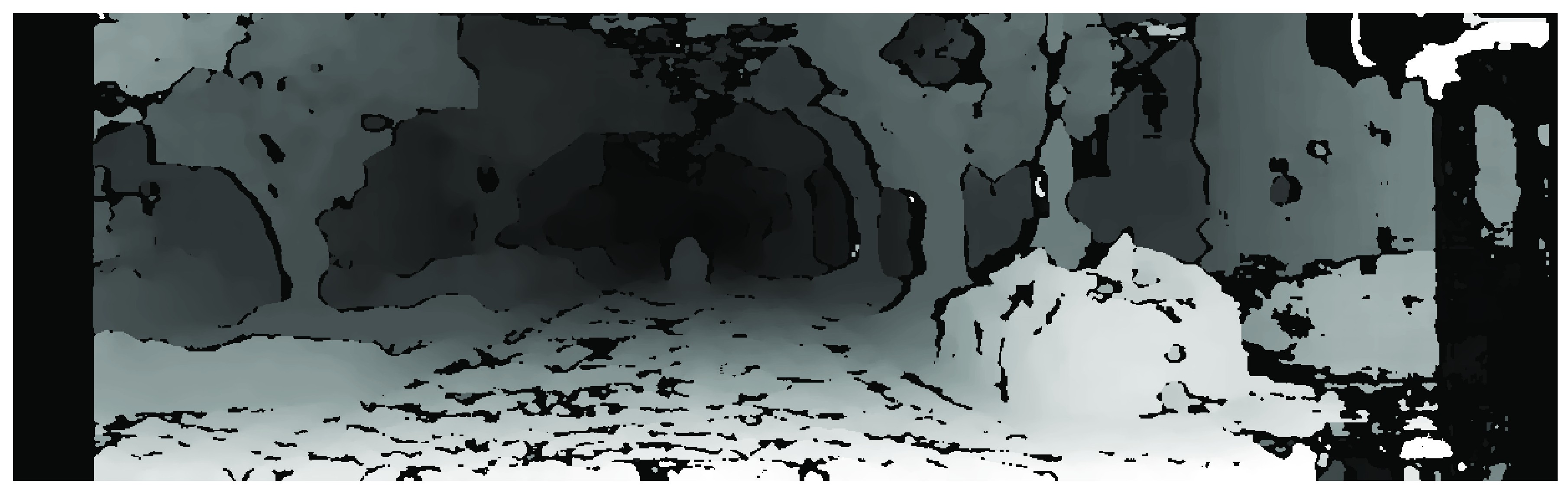
Given a pair of images from a stereo camera, we can compute a disparity map. Suppose a particular 3D in the physical world \(F\) is located at the position \((x,y)\) in the left image, and the same feature is located on \((x+d,y)\) in the second image, then the location \((x,y)\) on the disparity map holds the value \(d\). Note that the y-cordinates are the same since the images have been rectified. Thus, we can define disparity at each point in the image plane as: \(\begin{equation} d = x_{l} - x_{r} \end{equation}\)

Block-Matching Algorithm

Disparity at each point is computed using a sliding window. For every pixel in the left image a 15x15 pixels wide window is generated around it, and the value of all the pixels in the windows is stored. This window is then constructed at the same coordinate in the right image, and is slid horizontally, until the Sum-of-Absolute-Differences (SAD) is minimized. The algorithm used in our implementation is an advanced version of this block-matching technique, called the Semi-Global Block Matching algorithm. A function directly implements this algorithm in MATLAB:

disparityMap1 = disparity(I1_l,I1_r, 'DistanceThreshold', 5);

Feature Detection

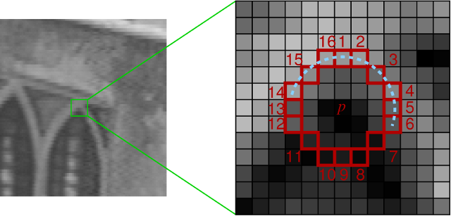
My approach uses the FAST corner detector. I’ll now explain in brief how the detector works, though you must have a look at the original paper and source code if you want to really understand how it works. Suppose there is a point \(\mathbf{P}\) which we want to test if it is a corner or not. We draw a circle of 16px circumference around this point as shown in figure below. For every pixel which lies on the circumference of this circle, we see if there exits a continuous set of pixels whose intensity exceed the intensity of the original pixel by a certain factor \(\mathbf{I}\) and for another set of contiguous pixels if the intensity is less by at least the same factor \(\mathbf{I}\). If yes, then we mark this point as a corner. A heuristic for rejecting the vast majority of non-corners is used, in which the pixel at 1,9,5,13 are examined first, and atleast three of them must have a higher intensity be amount at least \(\mathbf{I}\), or must have an intensity lower by the same amount \(\mathbf{I}\) for the point to be a corner. This particular approach is selected due to its computational efficiency as compared to other popular interest point detectors such as SIFT.

Another thing that we do in this approach is something that is called “bucketing”. If we just run a feature detector over an entire image, there is a very good chance that most of the features would be concentrated in certain rich regions of the image, while certain other regions would not have any representation. This is not good for our algorithm, since it relies on the assumption of a static scene, and to find the “true” static scene, we must look at all of the image, instead of just certain regions of it. In order to tackle this issue, we divide the images into grids (of roughly 100x100px), and extract at most 20 features from each of this grid, thus maintaing a more uniform distribution of fetures.

In the code, you will find the following line:

points1_l = bucketFeatures(I1_l, h, b, h_break, b_break, numCorners);

This line calls the following function:

function points = bucketFeatures(I, h, b, h_break, b_break, numCorners)
% input image I should be grayscale

y = floor(linspace(1, h - h/h_break, h_break));
x = floor(linspace(1, b - b/b_break, b_break));

final_points = [];
for i=1:length(y)
    for j=1:length(x)
    roi =   [x(j),y(i),floor(b/b_break),floor(h/h_break)];
    corners = detectFASTFeatures(I, 'MinQuality', 0.00, 'MinContrast', 0.1, 'ROI',roi );
    corners = corners.selectStrongest(numCorners);
    final_points = vertcat(final_points, corners.Location);
    end
end
points = cornerPoints(final_points);

As you can see, the image is divided into grids, and the strongest corners from each grid are selected for the subsequent steps.

Feature Description and Matching

The fast corners detected in the previous step are fed to the next step, which uses a KLT tracker. The KLT tracker basically looks around every corner to be tracked, and uses this local information to find the corner in the next image. You are welcome to look into the KLT link to know more. The corners detected in \(\mathit{I}_{l}^{t}\) are tracked in \(\mathit{I}_{l}^{t+1}\) Let the set of features detected in \(\mathit{I}_{l}^{t}\) be \(\mathcal{F}^{t}\) , and the set of corresponding features in \(\mathit{I}_{l}^{t+1}\) be \(\mathcal{F}^{t+1}\).

In MATLAB, this is again super-easy to do, and the following three lines intialize the tracker, and run it once.

tracker = vision.PointTracker('MaxBidirectionalError', 1);
initialize(tracker, points1_l.Location, I1_l);
[points2_l, validity] = step(tracker, I2_l);

Note that in my current implementation, I am just tracking the point from one frame to the next, and then again doing the detection part, but in a better implmentation, one would track these points as long as the number of points do not drop below a particular threshold.

Triangulation of 3D PointCloud

The real world 3D coordinates of all the point in \(\mathcal{F}^{t}\) and \(\mathcal{F}^{t+1}\) are computed with respect to the left camera using the disparity value corresponding to these features from the disparity map, and the known projection matrices of the two cameras \(\mathbf{P}_{1}\) and \(\mathbf{P}_{2}\). We first form the reprojection matrix \(\mathbf{Q}\), using data from \(\mathbf{P1}\) and \(\mathbf{P2}\):

\(c_{x}\) = x-coordinate of the optical center of the left camera (in pixels)
\(c_{y}\) = y-coordinate of the optical center of the left camera (in pixels)
\(f\) = focal length of the first camera
\(T_{x}\) = The x-coordinate of the right camera with respect to the first camera (in meters)

We use the following relation to obtain the 3D coordinates of every feature in \(\mathcal{F}_{l}^{t}\) and \(\mathcal{F}_{l}^{t+1}\)

Let the set of point clouds obtained from be referred to as \(\mathcal{W}^{t}\) and \(\mathcal{W}^{t+1}\). To have a better understanding of the geometry that goes on in the above equations, you can have a look at the Bible of visual geometry i.e. Hartley and Zisserman’s Multiple View Geometry.

The Inlier Detection Step

This algorithm defers from most other visual odometry algorithms in the sense that it does not have an outlier detection step, but it has an inlier detection step. We assume that the scene is rigid, and hence it must not change between the time instance \(t\) and \(t+1\). As a result, the distance between any two features in the point cloud \(\mathcal{W}^{t}\) must be same as the distance between the corresponding points in \(\mathcal{W}^{t+1}\). If any such distance is not same, then either there is an error in 3D triangulation of at least one of the two features, or we have triangulated a moving, which we cannot use in the next step. In order to have the maximum set of consistent matches, we form the consistency matrix \(\mathbf{M}\) such that:

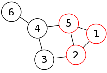
From the original point clouds, we now wish to select the largest subset such that they are all the points in this subset are consistent with each other (every element in the reduced consistency matrix is 1). This problem is equivalent to the Maximum Clique Problem, with \(\mathbf{M}\) as an adjacency matrix. A cliques is basically a subset of a graph, that only contains nodes that are all connected to each other. An easy way to visualise this is to think of a graph as a social network, and then trying to find the largest group of people who all know each other.

This problem is known to be NP-complete, and thus an optimal solution cannot be found for any practical situation. We therefore employ a greedy heuristic that gives us a clique which is close to the optimal solution:

1. Select the node with the maximum degree, and initialize the clique to contain this node.
2. From the existing clique, determine the subset of nodes \(\mathit{v}\) which are connected to all the nodes present in the clique.
3. From the set \(\mathit{v}\), select a node which is connected to the maximum number of other nodes in \(\mathit{v}\). Repeat from step 2 till no more nodes can be added to the clique.

The above algorithm is implemented in the following two functions in my code:

function cl = updateClique(potentialNodes, clique, M)


maxNumMatches = 0;
curr_max = 0;
for i = 1:length(potentialNodes)
    if(potentialNodes(i)==1)
        numMatches = 0;
        for j = 1:length(potentialNodes)
            if (potentialNodes(j) & M(i,j))
                numMatches = numMatches + 1;
            end
        end
        if (numMatches>=maxNumMatches)
            curr_max = i;
            maxNumMatches = numMatches;
        end
    end
end

if (maxNumMatches~=0)
    clique(length(clique)+1) = curr_max;
end

cl = clique;


function newSet = findPotentialNodes(clique, M)

newSet = M(:,clique(1));
if (size(clique)>1)  
    for i=2:length(clique)
        newSet = newSet & M(:,clique(i));
    end
end

for i=1:length(clique)
    newSet(clique(i)) = 0;
end

Computation of \(\mathbf{R}\) and \(\mathbf{t}\)

In order to determine the rotation matrix \(\mathbf{R}\) and translation vector \(\mathbf{t}\), we use Levenberg-Marquardt non-linear least squares minimization to minimize the following sum:

\(\mathcal{F}^{t}, \mathcal{F}^{t+1}\): Features in the left image at time \(t\) and \(t+1\) \(\mathbf{j_{t}}, \mathbf{j_{t+1}}\): 2D Homogeneous coordinates of the features \(\mathcal{F}^{t}, \mathcal{F}^{t+1}\)
\(\mathbf{w_{t}}, \mathbf{w_{t+1}}\): 3D Homogeneous coordinates of the features \(\mathcal{F}^{t}, \mathcal{F}^{t+1}\)
\(\mathbf{P}\): \(3\times4\) Projection matrix of left camera
\(\mathbf{T}\): \(4\times4\) Homogeneous Transformation matrix\

The Optimization Toolbox in MATLAB directly implements the Levenberg-Marquardt algorithm in the function lsqnonlin, which needs to be supplied with a vector objective function that needs to be minimized, and a set of parameters that can be varied.

This is how the function to be minimized is represented in MATLAB. This part of the algorithm, is the most computationally expensive one.

function F = minimize(PAR, F1, F2, W1, W2, P1)
r = PAR(1:3);
t = PAR(4:6);
%F1, F2 -> 2d coordinates of features in I1_l, I2_l
%W1, W2 -> 3d coordinates of the features that have been triangulated
%P1, P2 -> Projection matrices for the two cameras
%r, t -> 3x1 vectors, need to be varied for the minimization
F = zeros(2*size(F1,1), 3);
reproj1 = zeros(size(F1,1), 3);
reproj2 = zeros(size(F1,1), 3);

dcm = angle2dcm( r(1), r(2), r(3), 'ZXZ' );
tran = [ horzcat(dcm, t); [0 0 0 1]];

for k = 1:size(F1,1)
    f1 = F1(k, :)';
    f1(3) = 1;
    w2 = W2(k, :)';
    w2(4) = 1;
    
    f2 = F2(k, :)';
    f2(3) = 1;
    w1 = W1(k, :)';
    w1(4) = 1;
    
    f1_repr = P1*(tran)*w2;
    f1_repr = f1_repr/f1_repr(3);
    f2_repr = P1*pinv(tran)*w1;
    f2_repr = f2_repr/f2_repr(3);
    
    reproj1(k, :) = (f1 - f1_repr);
    reproj2(k, :) = (f2 - f2_repr);    
end

F = [reproj1; reproj2];

Validation of results

A particular set of \(\mathbf{R}\) and \(\mathbf{t}\) is said to be valid if it satisfies the following conditions:

1. If the number of features in the clique is at least 8.
2. The reprojection error \(\epsilon\) is less than a certain threshold.

The above constraints help in dealing with noisy data.

An important “hack”

If you run the above algorithm on real-world sequences, you will encounter a rather big problem. The assumption of scene rigidity stops holding when a large vehicle such as a truck or a van occupies a majority of the field of view of the camera. In order to deal with such data, we introduce a simple hack: accept a tranlsation/rotation matrix only if the dominant motion is in the forward direction. This is known to improve results significantly on the KITTI dataset, though you won’t find in this hack explicitly written in most of the papers that are published on the same!