Monocular Visual Odometry using OpenCV

Last month, I made a post on Stereo Visual Odometry and its implementation in MATLAB. This post would be focussing on Monocular Visual Odometry, and how we can implement it in OpenCV/C++. The implementation that I describe in this post is once again freely available on github. It is also simpler to understand, and runs at 5fps, which is much faster than my older stereo implementation.

If you are new to Visual Odometry, I suggest having a look at the first few paragraphs (before all the math starts) of my old post. It talks about what Visual Odometry is, why we need it, and also compares the monocular and stereo approaches.

Acquanted with all the basics of visual odometry? Cool. Let’s go ahead.

Demo

Before I move onto describing the implementation, have a look at the algorithm in action!

Pretty cool, eh? Let’s dive into implementing it in OpenCV now.

Formulation of the problem

Input

We have a stream of gray scale images coming from a camera. Let the frames, captured at time \(t\) and \(t+1\) be referred to as \(\mathit{I}^{t}\), \(\mathit{I}^{t+1}\). We have prior knowledge of all the intrinsic parameters, obtained via calibration, which can also be done in OpenCV.

Output

For every pair of images, we need to find the rotation matrix \(R\) and the translation vector \(t\), which describes the motion of the vehicle between the two frames. The vector \(t\) can only be computed upto a scale factor in our monocular scheme.

Algorithm Outline

1. Capture images: \(\mathit{I}^t\), \(\mathit{I}^{t+1}\),
2. Undistort the above images.
3. Use FAST algorithm to detect features in \(\mathit{I}^t\), and track those features to \({I}^{t+1}\). A new detection is triggered if the number of features drop below a certain threshold.
4. Use Nister’s 5-point alogirthm with RANSAC to compute the essential matrix.
5. Estimate \(R, t\) from the essential matrix that was computed in the previous step.
6. Take scale information from some external source (like a speedometer), and concatenate the translation vectors, and rotation matrices.

You may or may not understand all the steps that have been metioned above, but don’t worry. All the points above will be explained in great detail in the text to follow.

Undistortion

Distortion happens when lines that are straight in the real world become curved in the images. T his step compensates for this lens distortion. It is performed with the help of the distortion parameters that were obtained during calibration. Since the KITTI dataset that I’m using already comes with undistorted images, I won’t write the code about it here. However, it is relatively straightforward to undistort with OpenCV.

Feature Detection

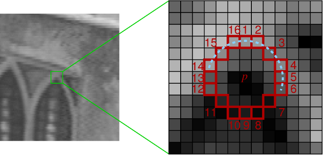
My approach uses the FAST corner detector, just like my stereo implementation. I’ll now explain in brief how the detector works, though you must have a look at the original paper and source code if you want to really understand how it works. Suppose there is a point \(\mathbf{P}\) which we want to test if it is a corner or not. We draw a circle of 16px circumference around this point as shown in figure below. For every pixel which lies on the circumference of this circle, we see if there exits a continuous set of pixels whose intensity exceed the intensity of the original pixel by a certain factor \(\mathbf{I}\) and for another set of contiguous pixels if the intensity is less by at least the same factor \(\mathbf{I}\). If yes, then we mark this point as a corner. A heuristic for rejecting the vast majority of non-corners is used, in which the pixel at 1,9,5,13 are examined first, and atleast three of them must have a higher intensity be amount at least \(\mathbf{I}\), or must have an intensity lower by the same amount \(\mathbf{I}\) for the point to be a corner. This particular approach is selected due to its computational efficiency as compared to other popular interest point detectors such as SIFT.

Using OpenCV, detecting features is trivial, and here is the code that does it.

void featureDetection(Mat img_1, vector<Point2f>& points1)	{ 
  vector<KeyPoint> keypoints_1;
  int fast_threshold = 20;
  bool nonmaxSuppression = true;
  FAST(img_1, keypoints_1, fast_threshold, nonmaxSuppression);
  KeyPoint::convert(keypoints_1, points1, vector<int>());
}

The parameters in the code above are set such that it gives ~4000 features on one image from the KITTI dataset. You may want tune these parameters so as to obtain the best performance on your own data. Note that the code above also converts the datatype of the detected feature points from KeyPoints to a vector of Point2f, so that we can directly pass it to the feature tracking step, described below:

Feature Tracking

The fast corners detected in the previous step are fed to the next step, which uses a KLT tracker. The KLT tracker basically looks around every corner to be tracked, and uses this local information to find the corner in the next image. You are welcome to look into the KLT link to know more. The corners detected in \(\mathit{I}^{t}\) are tracked in \(\mathit{I}^{t+1}\). Let the set of features detected in \(\mathit{I}^{t}\) be \(\mathcal{F}^{t}\) , and the set of corresponding features in \(\mathit{I}^{t+1}\) be \(\mathcal{F}^{t+1}\). Here is the function that does feature tracking in OpenCV using the KLT tracker:

void featureTracking(Mat img_1, Mat img_2, vector<Point2f>& points1, vector<Point2f>& points2, vector<uchar>& status)	{ 

//this function automatically gets rid of points for which tracking fails

  vector<float> err;					
  Size winSize=Size(21,21);																								
  TermCriteria termcrit=TermCriteria(TermCriteria::COUNT+TermCriteria::EPS, 30, 0.01);

  calcOpticalFlowPyrLK(img_1, img_2, points1, points2, status, err, winSize, 3, termcrit, 0, 0.001);

  //getting rid of points for which the KLT tracking failed or those who have gone outside the frame
  int indexCorrection = 0;
  for( int i=0; i<status.size(); i++)
     {  Point2f pt = points2.at(i- indexCorrection);
     	if ((status.at(i) == 0)||(pt.x<0)||(pt.y<0))	{
     		  if((pt.x<0)||(pt.y<0))	{
     		  	status.at(i) = 0;
     		  }
     		  points1.erase (points1.begin() + i - indexCorrection);
     		  points2.erase (points2.begin() + i - indexCorrection);
     		  indexCorrection++;
     	}

     }

}

Feature Re-Detection

Note that while doing KLT tracking, we will eventually lose some points (as they move out of the field of view of the car), and we thus trigger a redetection whenver the total number of features go below a certain threshold (2000 in my implementation).

Essential Matrix Estimation

Once we have point-correspondences, we have several techniques for the computation of an essential matrix. The essential matrix is defined as follows: \(\begin{equation} y_{1}^{T}Ey_{2} = 0 \end{equation}\) Here, \(y_{1}\), \(y_{2}\) are homogenous normalised image coordinates. While a simple algorithm requiring eight point correspondences exists\cite{Higgins81}, a more recent approach that is shown to give better results is the five point algorithm¹. It solves a number of non-linear equations, and requires the minimum number of points possible, since the Essential Matrix has only five degrees of freedom.

RANSAC

If all of our point correspondences were perfect, then we would have need only five feature correspondences between two successive frames to estimate motion accurately. However, the feature tracking algorithms are not perfect, and therefore we have several erroneous correspondence. A standard technique of handling outliers when doing model estimation is RANSAC. It is an iterative algorithm. At every iteration, it randomly samples five points from out set of correspondences, estimates the Essential Matrix, and then checks if the other points are inliers when using this essential matrix. The algorithm terminates after a fixed number of iterations, and the Essential matrix with which the maximum number of points agree, is used.

Using the above in OpenCV is again pretty straightforward, and all you need is one line:

E = findEssentialMat(points2, points1, focal, pp, RANSAC, 0.999, 1.0, mask);

Computing R, t from the Essential Matrix

Another definition of the Essential Matrix (consistent) with the definition mentioned earlier is as follows: \(\begin{equation} E = R[t]_{x} \end{equation}\) Here, \(R\) is the rotation matrix, while \([t]_{x}\) is the matrix representation of a cross product with \(t\). Taking the SVD of the essential matrix, and then exploiting the constraints on the rotation matrix, we get the following:

Here’s the one-liner that implements it in OpenCV:

recoverPose(E, points2, points1, R, t, focal, pp, mask);

Constructing Trajectory

Let the pose of the camera be denoted by \(R_{pos}\), \(t_{pos}\). We can then track the trajectory using the following equation:

Note that the scale information of the translation vector \(t\) has to be obtained from some other source before concatenating. In my implementation, I extract this information from the ground truth that is supplied by the KITTI dataset.

Heuristics

Most Computer Vision algorithms are not complete without a few heuristics thrown in, and Visual Odometry is not an exception. The heuristive that we use is explained below:

Dominant Motion is Forward

The entire visual odometry algorithm makes the assumption that most of the points in its environment are rigid. However, if we are in a scenario where the vehicle is at a stand still, and a buss passes by (on a road intersection, for example), it would lead the algorithm to believe that the car has moved sideways, which is physically impossible. As a result, if we ever find the translation is dominant in a direction other than forward, we simply ignore that motion.

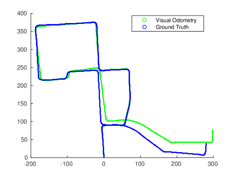
Results

So, how good is the performance of the algorithm on the KITTI dataset? See for yourself.

What next?

A major limitation of my implementation is that it cannot evaluate relative scale. I did try implementing some methods, but I encountered the problem which is known as “scale drift” i.e. small errors accumulate, leading to bad odometry estimates. I hope I’ll soon implement a more robust relative scale computation pipeline, and write a post about it!