Recognizing Human Activities with Kinect - Choosing a temporal model

Update: I have posted the sequel to this post here

In this blog post, I will very briefly talk about some popular models used for temporal/sequence classification, their advantages/disadvantages, which one I used for my human activity recognition project, and why. This post is intended for people who would like to delve into sequence classification, but don’t know where to start. I plan to follow up on this post with another post that explains in detail our implementation of recognizing human activities from RGBD data. However, if you want to have a look at it now, here are the slides.

In one my graduate-level course Machine Learning for Computer Vision, we were asked to select a research paper to review and present. We selected the paper Unstructured Human Activity Detection from RGBD Images. Our reasons for this selection were several: it was fairly recent (2012), had a large number of citations (according to google scholar, at least), and it dealt with sequential data (RGBD videos). Temporal models, or sequence classification, was something that was not covered in our course, and so we were eager to explore this area of Machine Learning. We read the paper, made a poster out of it, and presented it to our peers, TAs and the professor.

The next part of the course was more interesting, and it involved us picking up a Machine Learning problem, and we then had the option of either implementing an existing approach to the problem, or we could come with our own approach to solve it. We could have implemented the paper that we reviewed, but it seemed to more interesting to have a look at the models available for sequence classification, and then use one such model for our problem.

So we started looking around, and found that that following three models (and their variations) seem to be the most popular:

1. Hidden Markov Models (HMMs)
2. Maximum Entropy Markov Models (MEMMs)
3. Conditional Random Fields (CRFs)

Here’s the very basic intuition about temporal models: Suppose you are reading some text character by character. The first character that you observe is an “i”. Now, what do you think are the chances of you observing another “i”. Pretty slim, right? This is because consecutive “i” are pretty rare while reading english text. Modeling such probabilistic relationships in a mathematical form is precisely why we use temporal models, instead of just using some regular classifier (such as logistic regression). There’s two more popular models for sequential classification (or structured prediction, as some people like to call it), and they are: 1) Structural SVM, 2) Recurrent Neural Nets. I won’t talk about for either of them, as I have not used them, but you are welcome to check them out.

Hidden Markov Models are the oldest, and have been used in things like speech-to-text since the 1960s. MEMMs came around in 2000, only to be followed (and overshadowed) by Conditional Random Fields an year later. Both MEMMs and CRF came from the Andrew McCallum’s research group, and were focused on Natural Language Processing tasks. However, once you have extracted features from sequential data, you can use these models as long as your features satisfy the assumptions made by these models. Note that all of these models are special cases of probabilistic graphical models, so all the inference and learning algorithms from there can directly be applied here.

Hidden Markov Models

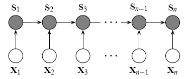
As I mentioned earlier, Hidden Markov Models have been around for a long time, and were heavily used by the speech processing community. I won’t much into the details/code of HMMs, as there are a large number of resources that describe the topic, targeted both at beginners and those who want to go into all the details. HMMs are generative models, and efficient dynamic programming algorithms are available for both training and inference. The models uses hidden states, and assumes that the observed states are independent of each other, given their hidden states. A common way to go about doing classification with HMMS is the following: Train an HMM for every class, and then for every new example, find the probability of that example being generated by each HMM, the HMM that gives the maximum probability is your final class.

However, with HMMs come a number of disadvantages, with the major ones being:

1. Requires enumeration of all possible observation sequences.
2. Requires the observations to be independent of each other (given the hidden state).
3. Generative approach for solving a conditional problem leading to unnecessary computations.

Maximum Entropy Markov Models

So, let’s move onto a new model, which, in theory, solves all of the above problems: MEMMs. MEMMs were introduced in 2000, and were at that time used in NLP tasks, and showed improvements in tasks where assumption [2] mentioned above was not true. MEMMs are discriminative models, so they also do away with problems [1] and [3]. There’s also a hierarchical version of the same model, and a Hierarchical MEMM is what was used in the paper that we reviewed. The paper contains an interesting way of selecting graph structure, and I recommend checking it out.

But along with MEMMs comes it’s own problem, commonly called as the label-bias problem.

Label bias problem

1. States with low-entropy transition distributions ”effectively ignore” their observations. States with lower transitions have ”unfair advantage”.
2. Since training is always done with respect to known previous tags, so the model struggles at test time when there is uncertainty in the previous tag.

It is impossible to understand the above without some background on what MEMMs are, so it is advisable to first look at how MEMMs work , and then at the original CRF paper which talks about the label bias problem.

Conditional Random Fields -> Star of the show

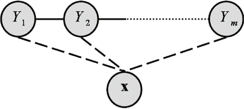
To overcome the label-bias problem of MEMMs, CRFs were introduced an year later, and demonstrated superior or equivalent performance in almost every NLP task that the authors tested it on. CRFs (and its variants) are considered as state-of-the-art in a number of machine learning problems, specially in Computer Vision. They are used not only for temporal modeling, but can also model more complicated relationships in high-dimensional data, and some applications include image segmentation and depth estimation from monocular images. Understanding CRFs is a little more challenging than HMMs or MEMMs, so I will list a few resources for you to get started with. For beginners, the best resource is this short course by Charles Elkan. It also has accompanying course notes, and if you go to this guy’s academic website, you can also find some programming assignments to implement CRFs. Here is a more comprehensive list of resources related to CRFs, and it’s pretty thorough.

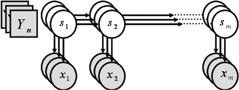
Now, in 2006, there was an extension to CRF by the MIT CSAIL lab, called hidden CRFs. Here is the original paperoriginal paper. What this does, in essence, is to introduce another layer of hidden states, and is designed to assign a single label to every sequence. This is different from MEMMs and CRFs, which assigned a label to every observation in a sequence, and different from HMMs too (wherein a stack of HMMs was trained for classification).

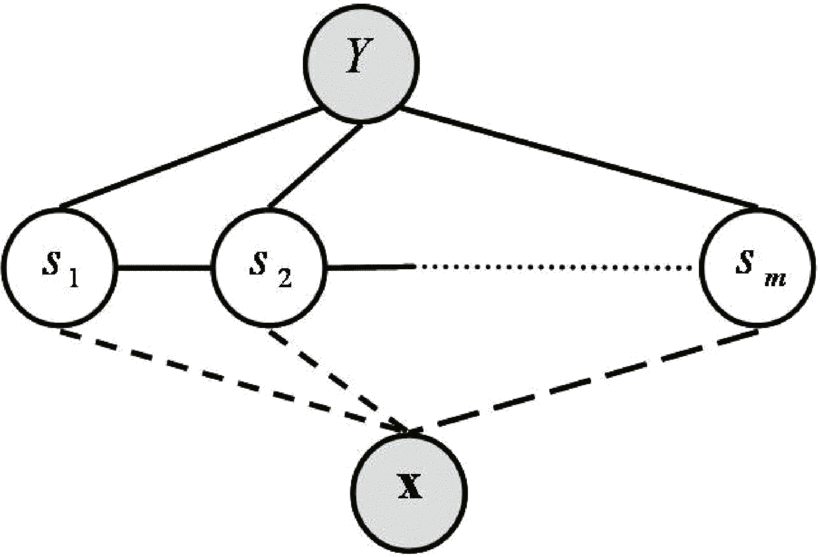
The original hCRF paper applied it to gesture recognition from RGB videos, and demonstrated superior performance to CRF in classifying gestures, so we zeroed down on this model, to be used for our Human Activity Classification task (note that activities are not exactly the same as gestures).

The real icing on the cake was this-> MIT CSAIL had released a well documented toolbox, making it ridiculously easy for us to use this model on whichever dataset that we wanted, and the only major programming part that was left to us now was was the feature extraction stage.

In a future blog post, I will describe in detail the implementation of our project: the dataset, the features we used, and what results we got.